Navigation at UW Eau Claire Priory

Figure 1

Figure 2

Introduction

       This final exercise involved working with navigation and took place out at the Eau Claire Priory which is about 4 miles south of the University. Earlier in the semester, each students made a navigation map of this area. The best map was selected from each group and used with a compass and a back up GPS to mark 5 of the points on the navigation course on the property. Figure 1 to the left displays the locations that were assigned to group 2 by professor Joseph Hupy. Figure 2 to the right shows the device that was used in connection with the bad elf app that was downloaded prior to class. This device was used to track the students as they went throughout the lab and it showed a detail track log. The first step after receiving the navigation maps from earlier was to manually plot out the points on the map and to label them, in order to get the bearings of where to start and finish the exercise.

Figure 3

Figure 5

Figure 4

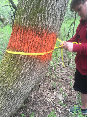
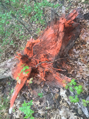
           Figure 3 to the upper left shows the GPS that was used to navigate the priory. This proposed somewhat of a problem due to the steep terrain of the Priory property, as the hills caused a few loses in satellites. Figure 4 is the location marking tape that was used and figure 5 shows the location marking spray paint that was used to mark a band around the tree at tree height to assist groups that will be completing the navigation course at other times.

Figure 6

        Figures 6-9 show the process of marking the navigation locations, which are trees. The spray paint was put about 10 inches thick around chest height for easy visibility. The navigation to the trees was done using Google Maps, the compasses on the students phones, the Bad Elf GPS and the Garmin GPS.

Figure 7

Figure 8

Figure 9

Surveying Point Features using High Precision GPS

Introduction

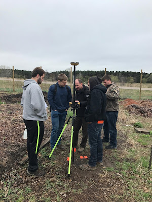
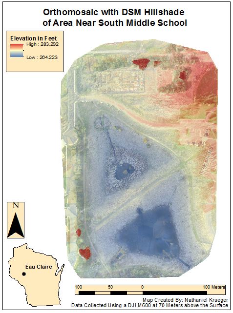
        The purpose of this lab is to be able to gather a number of different variables of data including temperature (C), pH levels, and soil moisture at various points throughout the the public use gardens that are located near Eau Claire South Middle School. At each point of data collection a flag was put in and a GPS location was recorded. The grid system that was used was not set in stone and it was made by the class, the goal was to learn how to collect the data accurately more so than measuring out a uniform grid pattern. A survey grade Dual Frequency GPS was used to record data as well as take the specific coordinates of each data recording point. Throughout this lab there was a number of tools and equipment used, including the GPS, pH meter, soil thermometer, flags to mark the points, and finally distilled water to clean the pH meters between each soil sample reading. This data collection is the start of what will be a two part lab, the second part of the lab will include UAS aerial imagery.

Study Area

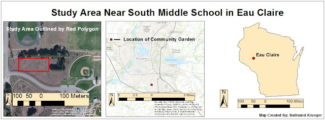
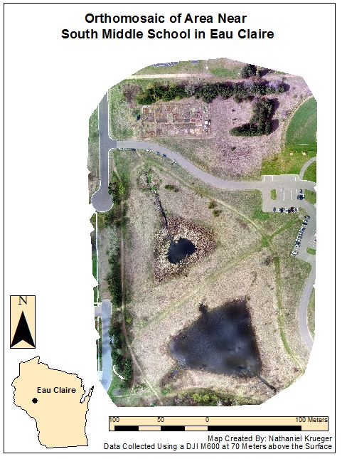
        Figure 1 below is a number of maps that show the study area for the data collection in this exercise. The area of interest (AOI) is located to the south of the Eau Claire South Middle School, just to the north of Pine Meadow Golf Course, and to the southeast of the corner of Mitchell Avenue and Hester Street. Data collection took place on April 26th, the temperature was in the mid 40's and the rain had just ceased after the Eau Claire area got over a half inch of rain. With the exception of a few garlic plants, grass and some weeds, the majority of the community garden was rather bare, which made for muddy conditions.

Figure 1

Methods

        The data points collected throughout this lab were done so at sub meter accuracy, using a GPS system that at time of purchase was over $12,000. Before data collection began, Proffesor Hupy demonstrated how to calibrate the pH meters, as they had just arrived that day. Next, volunteers were taken to operate the GPS unit, which has many capabilities including data records of the values collected. Next a student was selected to record the data values on paper to ensure that the data matched with the data being recorded on the GPS. Two students went ahead of the rest to place the flags in a grid pattern and to begin the data collection with the pH meter. Some groups of students used the TDR, other used the pH meter and some used the soil thermometers. Students were encouraged to try each device to become familiar with every aspect of the data collection.

          One group of students operated the GPS, another used the soil thermometer, and two groups of students recorded data using the pH meter. As stated in the introduction, there was no set in stone requirements of flag placement, but rather just a rough grid pattern. The flags were placed in semi straight lines that ran east to west, once at the west end the data collection headed back east. For the most part the flags were equal distances apart as well as the distance between rows. Some of the plots appeared to be tilled, so there was an effort to stay out of those plots. Additionally, Professor Hupy has garlic plants planted on the north side of the plot in the middle, and he wanted a few readings in the plots to see the overall soil quality of the area near his plants, this explains the north side row of data collection.

Figure 2

Figure 3

     
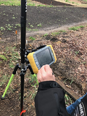
         Figure 2, above left shows a close up of the survey grade GPS that was used to obtain sub centimeter accuracy for this lab. The device is not hard to use, but there is a large amount of settings and useful features that do take some time to become comfortable with. This was the longest data recording process of the day, as the user needs to navigate to a few different screens at each data collection point. Figure 3 to the left shows Professor Joesph Hupy showing students how to use the GPS. The survey grade GPS was used to get a coordinate at sub centimeter accuracy, after the location was recorded the group operating the device also had to enter in the temperature, soil moisture and pH for that point. The data recorder is pictured on the left side of figure 3, and he was responsible for recording all the data and conveying it to the group entering it into the GPS system.

Figure 4

Figure 5

        Figure 4, displayed above shows a student taking a temperature reading of the soil. The device takes a temperature reading by simply sticking the metal end of the device into the ground and letting the temperature became consistent at one number. Between each temperature reading a simple wipe of the stick to remove previous soil was all that was required. A few times this device took some time to get a reading, whereas when it was in the air and not in soil it would always register. When the device would display an error message the pH meter was used to record the temperature for that point. Figure 5 above right shows the collection process for the pH meter. A soil sample was taken in the small plastic container and distilled water was added to the tube, then the cover was placed on and the sample was shook in an effort to mix the water and soil so the meter could get a reading. The readings took about 30 seconds each to get a number that was not changing. After each soil collection point the meter needed to be rinsed with distilled water along with the tube used for the soil samples. Normally this process would not take to long, but the squirt bottle decided not to squirt on this day so the meter and collection tube were cleaned manually by dumping the water. This slowed the process until Professor Hupy provided an additional working squirt bottle.

Figure 6

Figure 7

         Figure 6 above is a close up of the pH meters that were used. A temperature reading is displayed at the bottom of the screen and the pH value is displayed in the center of the screen. This process of data collection was very simple, though cleaning the device between each soil reading was a bit redundant. Figure 7 to the upper right shows the  TDR device that was used to record the soil moisture content. This device records soil moisture by sending an pulse between the two metal conductors that go into the soil. Being that the day of data collection was very moist from all the rain received in the previous 24 hours, it would be interesting to go back another day when there was not fresh precipitation. There was only one device available for this step so three readings were taken at each flag and the average was recorded. This is in contrast to the steps taken with the pH meter, as there were two groups recording the pH to ensure data quality.

Results

        

Figure 8

Figure 9

Conclusion

       In conclusion, the survey grade GPS unit that was used was very accurate and allowed for very precise locations of the data collection points. A number of data collection devices were used throughout this lab. In order to replicate this lab outside of the class setting, it would be very costly, as the GPS was nearly $12,000 when originally purchased. Though the unit has many capabilities, and could be used for countless other applications that could benefit an individual or company. In total data was collected for about two hours, and there was an additional set up and clean up time on top of that two hours.
       

Arc Collector Part II: Bumper Stickers

Introduction

           This lab required a more sophisticated understanding of Arc Collector then the previous exercise, including how to set up the software and then collect data. This lab was much more elaborate than the introductory Arc Collector assignment and required the class to come up with unique study questions that could be answered by collected data in the form of points with attributes, with at least one of the attributes involving a numeric field. For this lab the connection between bumper stickers and automobiles will be explored. More specifically, the data collected sought to see if there was a relationship between the year of a car and the number of bumper stickers, as well as the type of bumper sticker. Additionally, the idea that a type of vehicle being a car, SUV or truck might determine the type of bumper stickers on the vehicle was explored.

        The study area for the data collection took place on the University of Wisconsin Eau Claire, to the south of Philips and Davies hall in the Davies parking lot. In total 122 vehicles and there bumper stickers or lack there of were recorded. This was done because it was a convenient location that was a wide age range, as the university was a wide spread of ages. Replicating this data collection in different parking lots around town would most certainly show different results. Data collection was conducted on April 25th from 10 am until 12:30 am. Setting up the project correctly in Arc Catalog is the first step to successful and accurate data collection. If a step is skipped or a value is displayed incorrectly, data integrity could be hindered.

Figure 1

       
         Figure 1 above shows the how the data points looked when they were collected in the Arc Collector map. They were not even remotely accurate as the GPS was likely having troubles getting a good signal due to the large hill located to the south and the tall buildings to the north. Each data point was collected directly behind the cars in each stall to ensure that all the stickers of the rear of the car were clearly visible. Once the data was opened in ArcGIS online the points were corrected to where they were actually taken.

Figure 2

            Figure 2 above shows the corrected data collection points. The points were corrected by simply clicking and dragging in ArcGIS online.

Figure 3

        Figure 3 above shows the study area in greater detail as highlighted by the red box. The Davies center and Philips hall are shown to the north of the data collection area. The specific area was the middle two rows of parking in the Davies parking lot, the outside rows were not done due to time constraints and the time that took to collect nearly 500 attribute values for the 122 data points. 

Methods

         The process of setting up Arc Collector begins with setting up a geodatabase, and then selecting domains that are applicable to the data collection as well as setting up the feature class. In total there were four domains created in the database properties. The domains were type of bumper sticker, age of vehicle, type of vehicle and number of bumper stickers. The type of bumper sticker had 6 different codes, religious. sports, outdoors, political, other or none. For the age of the vehicle a short integer was selected, then for type of vehicle, car, SUV and truck were the three options. Finally the number of bumper stickers was set up, with values from 0 to 15, though no car displayed more than 7 bumper stickers during data collection. Next, the sign in to ArcGIS online was done using the UWEC enterprise account. The set up was shared in the form of a map, which made it accessible on the mobile devices. Tags were added so the project could be found by others, the tags being Geog 336 and bumper stickers. After this was set up, the project was published. From here the data can then be collected using the mobile app.

          The question that was sought to be answered by doing this data collection was whether or not the age and type of vehicle have a relationship to the number and type of bumper stickers that one has on there car. To deploy a data collection for this question, Arc Collector was used, which is a very user friendly, real time way to collect and upload data. Figures 4-9 are screenshots of the program in action that display how each of the different attributes appeared when being collected.

 

Figure 4

Figure 5

Figure 7

Figure 6

     Figure 4 to the right shows what the initial screen appeared as each time a car was selected for data collection. Every car that was in the Davies parking lot in the middle section was collected, none were skipped. The reason for some holes in the data is because there were no cars in the parking spots. Figure 5 to the right shows what the screen displaying the type of vehicle looked like. It states that the vehicle is either a car, truck of SUV. Figure 6 to the left shows the attribute displaying the age of the vehicle. As stated, the value was collected according to the number of years old the vehicle appeared. In order to get the actually age of the vehicle the owners would most likely have to be present of an extensive amount of research would have to be done about the cars. The reason a rough estimated was used was because of time constrains as well as the fact that it was not highly important to answer the question. Figure 7 to the right shows the attribute with the type of sticker. Either religious, sports, political, outdoors, or one that does not fall under any of the predefined categories. A car that recorded a no value were cars that did not have any type of stickers displayed.

Figure 9 above shows the corrected data collection points on the device they were collected on which was an iPhone 6. The quality is rather good and the points show up nicely.

Results

         Below are a series of maps that show the attributes that were collected throughout this exercise. Figure 4 below shows the estimate of the ages of the vehicles that were in the Davies parking lot at the time of the data collection. The was this is set up is that the ages 2-5 mean the vehicle is within 2-5 years old, while 6-8 means the vehicle is 6-8 years old and the same for 9-16. These were just ball park estimates which factored in a large knowledge of cars. It is important to note that if the data collection was done again, this field would be fixed to display the values in years, for example 2000-2005. An error was made when setting up the project and it was not realized until data collection began. Though this was not ideal it still gave a good idea of what the age distribution of the cars in the Davies parking lot were.

Figure 8

         Figure 5 below displays the type of vehicle that were recorded, being either a car, SUV or truck. Only five of the vehicles of the 122 in the data were trucks. This number is very low, though it is to be expected as gas is not cheap and a good percentage of the people parking in this lot are likely college age students, though there are exceptions. 84 of the 122 vehicles were cars, while 33 were SUV's and as stated above only five were trucks. This makes sense that a large majority of the vehicles were cars because they are cheaper and more fuel efficient.

Figure 9

          Figure 6 below is a map that displays the types of bumper stickers that were recorded. Surprisingly only 30 of the vehicles did not have bumper stickers, 7 were outdoor themed, 11 political, 6 religious, and 15 were sports related. The largest number of vehicles fell in the category of other, meaning that there was not a pre designated category that they fell under. 53 cars had stickers in the other category, if the data collection was re structure for use another time, some of the other categories would be added to get a more accurate reading on what people use for bumper stickers.

Figure 10

        Figure 7 below shows the number of bumper stickers that each car had. 50 of the vehicles only had 1 bumper sticker, which is just over just over 40 percent of the vehicles. This is likely because not many people want to degrade the look of there vehicle, but still want to show what there hobbies or views are, hence why one sticker was the most popular. 24 vehicles had 2 stickers, while 10 had 3.

Figure 11

     


          Throughout this lab there was a number of different things that were learned and that would be implemented if the exercise was done again in greater detail. After completion of the lab it was clear that the categories set up for collection were not the most popular bumper stickers. First and foremost a large majority of the vehicles that only had one bumper sticker were sticker of the dealership the automobile was purchased at. This was not thought about prior to completion and it should definitely be a category of bumper sticker if the lab was replicated. Also, a family category would be added that would include stickers such as "baby on board," of which there was more than five, as well as stick figure families, of which there was also a considerable amount. With a few simple corrections this lab could have shown more of the relationship with the fact that many of the newer cars only had the sticker showing where the car was bought. An example of this can be seen below in figure 14, this car had no additional bumper stickers other that the one that advertises the place it was bought.

Figure 12

Conclusion

        In conclusion, there is no notable association between the age or type of a vehicle and the number or type of bumper stickers on the vehicle. The number of bumper stickers varied from none to seven and did not show an association to the age or type of vehicle. In the beginning of the lab it was thought that older vehicles would have more bumper stickers under the premise that owners of new cars would not want to put bumper stickers on a new car. It was also thought that vehicles such as trucks and SUV's would have more outdoor bumper stickers, this was also disproved in this lab, though the sample size was small and there can not be a definitive relationship established for anywhere but the parking lot of Davies during data collection.

Arc Collector Weather Data Collection

Introduction

          The purpose of this lab is to become familiar with gathering geospatial data on a mobile device using Arc Collector. The purpose of using Collector is the fact that smartphones have more capabilities than most GPS units, that being said there is no reason to not be familiar with collecting data using it. Additionally smartphones can access online data in real time and allow the user to gather on the fly and upload data instantly. Additionally photos of the study areas can be uploaded instantly, this helps give the data viewers an idea of where the data was collected.
           The study area for this exercise was on the University of Wisconsin Eau Claire. The class was split up into seven groups and each group was assigned as area, a map showing the seven different data collection areas is displayed below in figure 1. The study area that will be discussed in this report is area seven, which was the study area that was assigned by Professor Joseph Hupy. Each group member was to collect around twenty data points and the group members were instructed to split the zones up into smaller areas to ensure that data was collected evenly throughout the assigned area. Data collected for this lab was on Wednesday, March 29th between 3:30 and 5:00pm. The attributes that were collected in this lab were temperature, dew point, wind chill, wind direction, wind speed, time, and group number. There was also a notes section available, though there were a few issues experienced with that and they will be discussed later in the results section.

Figure 1

Methods

          Arc Collector is a very straight forward method of data collection. For this exercise the data collection table was set up previously by Professor Joseph Hupy and the data recorded was entered and then submitted online where all other groups could see the data points and data recorded at those points. The attributes were selected by professor Hupy and that was done by creating feature class within the geodatabase.

Figure 2

          Figure 2 to the left shows the pocket weather meter that was used to record the weather data for this lab. This instrument has many uses, as it collects temperature, wind chill, dew point, wind speed and it also had other features that were not recorded. When in the field the points for weather collection were random, the only stipulation was that the data collection points were spread out within reason. While collecting data the points were instantly displayed after submitting the points, also as the data collection progressed the more points from other groups were also visible. Figure 3 to the bottom left shows what the screen looked like after opening the app, from there the white plus was clicked on in the top center. From there Figure 4 below shows what the data collection screen looked like. The data being collected was abbreviated, GRP is group number, TP is temperature, DP is dew point, WC is wind chill, WS is wind speed, WD is wind direction, then notes and time are the two final attributes. The white symbol of a camera in the upper right was used to attach photos.


       

         As far as units go, the temperature was recorded in degrees Fahrenheit, as well as the dew point and wind chill. Wind speed was recorded in miles per hour (MPH) and the wind direction was recorded in degrees and entered as a number from 0-360. The time was entered in military time from 0-2400 and it was important that there was no semicolon between the numbers in the time.
        From here a number of maps were made that displayed the data that was collected. ArcMap 10.4.1 was used. The temperature, wind chill, and dew point maps were all interpolated using the IDW tool to give a better idea of how those variables change with elevation.

Figure 3

Figure 4

Results


           Below in figure 5 is a map that shows points at which the weather data was collected. With the fact in mind that there was no specific place to collect points, the data points are reasonably evenly distributed. As discussed in the methods section, each student was to collect data at twenty different locations.

Figure 5

         Figure 6 below is a map that shows the points collected by each group, very similarly to figure 5, though figure 6 shows how close each group got to the other groups areas. For example, the data collectors in group seven had a point collected that was very near group six, this could be explained from a possible error in GPS because of the hill, or the data collector was slightly off. Group one did a nice job of covering the northern side of there area, they made sure to record data at both the northeast and northwest corners. Group five should have covered a much larger area in the southern third of there study area. At first glance it appears the group only covered about 60% of there assigned area. Certain groups such as group four were very limited on where there data points could be recorded as there is a lot of buildings in there study area.

Figure 6

        Figure 7 below is map of the wind chill that was interpolated using the IDW tool in ArcMap. The study area on the west of the map has a high wind chill, this can be explained because that location is the top of the hill, therefore the wind hits the exposed area much stronger. The lowest wind chill recorded was 45.0592 degrees and the highest recorded was 62.892 degrees. The area in the southeast portion of the map had the warmest wind chills, likely because the wind was out of the northeast and it was blocked by Philips hall which is to the northeast of the data collection there. 

Figure 7

          Figure 8 is a map that shows the direction of the wind along with the speed in miles per hour. The wind direction is shown by the way the arrows are pointing. The bridge is a good place to look to get an accurate wind direction, all of the arrows are point to the southwest, which means the wind direction was from the northeast. Variations in the wind direction on campus can be accounted for because of the buildings. Wind tunnels can be created as the wind hits the side of buildings and funnels ways that it was not actually blowing.

Figure 8

          Figure 9 below shows the dew points collected throughout the lab. The lowest dew points recorded were 30.0257 degrees and the highest recorded were 57.9726. Almost all of the high dew points were recorded on lower campus in lower elevation areas. In comparison the east side of the study areas were almost exclusively done on upper campus which is a much higher elevation.

Figure 9

         Figure 10 below is a map displaying the temperatures that were recorded. There are some warm spots on the north side of the Chippewa river, in contrast there are a few cold spots in the south portion of the study area near the towers halls.

Figure 10

       

           It would be interesting and beneficial to complete this exercise again and to collect all the data with one or two data collectors in order to ensure that the data was all collected the same way. Much of the variation in wind speeds and temperatures could be because the collectors did not let the units get an accurate reading.




Conclusion

           In conclusion, Arc Collector was a very useful method of data collection. It is very efficient, easy to use and allows a number of users to collect data and report it in real time. This lab demonstrated that a smartphone or tablet can indeed do all of the operations that a GPS can when used correctly. It was very useful to see the data collected displayed in real time. One issue that would need to be resolved if this was a data collection for company is making sure that each data collector is clear on how to collect the data. To clarify, some students entered time the wrong way, also some were not familiar with recording wind directions and finally not everyone held the meter long enough for it to get an accurate reading on wind speed. As professor Hupy discussed before data collection, as our supervisor he could see where all the students were during class time, assuring that no one was skipping out. This is applicable in the real world because an employer could track down time and ensure that employees stay on track, which saves time and money.

Distance Azimuth Survey

Introduction

          For the most part, the majority of surveying is done with the use of extremely accurate GPS technology coupled with survey stations. There may come a point in any geographers career where that technology may not be accessible or it could even fail completely. This lab focuses on building a skill set that can be used in many different settings and could be a real selling point to future employers. The purpose of this lab is to be able to create a survey using the distance and azimuth technique. This is a technique that is not very technical and it is only feasible on a reasonable scale and the accuracy will not be that of a GPS. Using low tech options assures that if ever faced with unfortunate circumstances, data will still be able to be collected. A distance azimuth survey is an implicit survey technique. Implicit survey data means that the data was collected relative to a know GPS coordinate. In contrast an explicit form of data collection means that there will be specific geographic locations.

          This lab took place in Putnam park, just to the south of the University of Wisconsin Eau Claire. The area where the lab was conducted was fairly heavily wooded, with exception of the jogging trail that runs through the park. A GPS unit was used to get three specific locations where a sample of ten trees was taken and the distance from the GPS point to the tree was recorded, along with the azimuth (degree) which gives the direction the tree is from the GPS point. Additionally the diameter of the trees was recorded. Each of the three survey locations were within 150 meters of each other, roughly 50 meters apart, though the distances were not measured. From there 10 trees were selected that had a clear line of sight from the reference point in which one group member stayed at all times until the survey was complete. The tools used for this lab include a GPS for reference point location, a notebook for data recording, a tape measure that calculates the diameter of the tree by taking a measurement around the tree at chest height and a compass for the azimuth. The tools used to record distance include laser distance finders and a more basic meter tape in an effort to get exposure to multiple data collection methods.

Methods

Figure 1

          The survey area was in Putnam park, south of UWEC roughly 150 meters away. This lab can not be completed without first understanding how each of the tools work, Professor Hupy offered assistance in explaining the uses of each of the devices. From there the first step in the lab is to use the GPS unit to get the coordinates of the reference point that was used, the reference point being where the group member will stand to get distance measurements along with where the tree is in association to the reference point using the azimuth tool. From here 10 trees were selected that offered a clear line of site to where the GPS coordinates were recorded. It is essential to note that the person who is on the GPS coordinate should not move at all because that will helps with data integrity. A table was made for each of the three locations, each table included latitude, longitude, distance, azimuth, and diameter. In the first station the distance and azimuth were both recorded using the TruPulse laser which is shown to the left by figure 1. This is done by simply pressing the black button on top of the handheld device, as noted before it is essential to make sure that the line of sight is clear or there could be interference with the laser. By using the arrows on the side of the laser the user can scroll through the setting to select distance and then degrees. Finally. the diameter of the trees should be collected at chest height. This was the least hands on of the three approaches. Figure 2 that is located to the bottom left shows the GPS unit which is pictured in the bottom of figure 2 and the tape measure used to measure the trees circumference is pictured in the top of figure 2.

Figure 2

          Area two was down Putnam trail to the east of the initial survey area roughly 50-75 yards. With the same steps as the first location the GPS was used to get a base point where one of the group members stood until the entire survey was complete. Again, ten trees were chosen at random and again the line of sight from reference point to trees must be clear. This time the azimuth was recorded using a tool that is called an azimuth compass. Next the distance from reference point to tree was measured using a meter tape. The azimuth compass is very easy to use, basically the same manner as the laser range finder, the point and shoot method. Again, the diameter of the trees was collected at chest height.

Figure 3

           Area three was roughly another 50-75 yards further east down the trail from the second survey area. The first step yet again is to get an accurate GPS location and to then have one group member stay in exactly that spot for the duration of the survey in area 3. Next, 10 trees should be selected for surveying. In this survey location the Sonin sound wave device was used to record the distance from the reference point to the trees. The device is used by the person on the reference point point at the another part of the device that another group member was holding up against the target trees. A sound wave is sent from one device and back to the other and a distance is registered. The diameter of the tree was then again recorded using the same method of hooking the tape around the tree at chest height, the method for getting the tree diameter is shown by figure 3 to the right. The azimuth was recorded using a good old fashioned compass, this is to show that many different methods can provide the same results. Figure 4 below shows the method that was used in the third survey area to record the distance. It is important to note that the tape measure was pulled tight before a measurement was taken, in order to ensure data integrity.

       

Figure 4

            After the field work for the distance azimuth survey was complete, the data was entered from the notebook in Microsoft Excel. It was essential to make sure that the data was normalized before adding the data into ArcMap. It is important to note that distance was in meters, azimuth is measured in degrees, not degrees minutes seconds, and the diameter of the trees was measured in centimeters.

       Once the data is normalized, it is ready to be brought into ArcMap. The data was brought into ArcMap using the 'Bearing Distance to Line' tool. Once the tool is open it asks for the lat and long, the distance, azimuth and diameter all collected during the survey. This tool does not create point, rather just the lines that represent the distance from the reference points to the trees. Next, using the 'Feature Vertices to Points' tool, points were created on the actual locations of the trees. Essentially this tool put points at the end of the lines that were just created using the previous tool. Once both these tools were ran, the result is lines and points that represent the distance and azimuth.


          It is important to note that even when working with less technology there can still be a number of issues that arise. When using both the Sonin and the TruPulse devices there needs to be a clear line of sight from the group member on the reference point to the tree being surveyed. This limited which trees could be selected and there is really no way around it without leaving the reference point which would skew the data. When using the TruPulse device if the user hit a twig that was closer than the tree, the distances could have been way off. Similarly it was important to make sure both members using the Sonin device held the devices at the same level, and that the person on the tree kept the device tight to the tree when readings were being taken. Additionally there was several mix ups with tools, people were not leaving there tools at the stations as they were instructed, but rather many carried them to the next survey area with them. This led to some confusion and some time lost, though it was not a major issue. Yet another issue was the lack of consistency when collected the diameter of the trees. Some group members are nearly a foot taller than other, so chest height for one group member is not chest height for another. This did not influence the data all that much, the reason the same person did not complete every tree was because they exercise was designed to get everyone involved in every aspect.

Results

          This lab was originally designed to have multiple maps because when they lab is conducted in the fall semester it is much easier to tell the tree type. For this lab in spring 2017 the tree type was not recorded. Truth be told there is not a ton of data to be displayed here so it will all be conveyed in one map. A table is included below as well to show how the data looked before being brought into ArcMap.

Figure 5

          Above in figure 5 is a map showing the sizes of the trees diameters. The point at which all of the point start is the reference point and the red lines are the lines that show the azimuth degree and also illustrate the distance from reference point to the trees surveyed. The largest tree in the survey was 148.20 centimeters, it was a very large tree that took two people to get around, this was done just to show some of the diversity in the tree sizes sampled. In contrast the smallest diameter tree was 6.80 cm, this was about the smallest tree that the tape would do, due to the way it has a few centimeters of blank tape. There is a fairly even distribution of the sizes of trees. Though it does seem that survey area 1 in the northwest corner has slightly smaller trees in diameter compared to the other two survey areas.

Figure 6

        Figure 6 is simply a map that shows the location of the trees without incorporating the diameters. Survey area 1 is in the Northwest corner of the map, survey area 3 is in the Southeast corner and survey area 2 is in the middle. Survey area 2 had a much smaller survey area, meaning the trees sampled were closer together, this was done because this was where the tape was used to measure distance. The other methods of finding distance were much easier, also keeping the tape measure trees close to the reference point ensure less bow in the tape and a more accurate distance reading.

         Figure 7 below is the table of the normalized data that was used to get the data displayed in ArcMap. The P_Number column shows which survey area was associated with which coordinates, this was done simply to help keep the data in the correct order and to make sure that there was no issues when bringing the data into ArcMap.

Figure 7

         One thing that hindered the map making process was the fact that survey are 1 which was to the far east of the map had an error when collected the GPS coordinates. When the data was brought into ArcMap the survey 1 area showed up half way up the hill, nearly 40 meters away from the actual on earth location. To remedy this issue the identify tool was used in ArcMap to find the coordinates of the actual location and then the excel sheet was fixed and the data was re brought into ArcMap. The reason for the poor GPS location initially is more likely than not from the large hill, there must not have been enough satellites connected to get an accurate location.

Conclusion

          In closing this lab has so many real world applications. An employer would be thrilled to know that if something happens to the technology, they still have someone in the field who can collect data. Distance azimuth surveying is actually very interesting and it really gives a sense of pride to the surveyor because it is not a machine doing all the work. This is a hands on approach that is relatively low cost, depending on the survey area size relatively low time and it is just all together a good skill to have.

Processing UAS Data in Pix4D

Introduction 

What is the overlap needed for Pix4D to process imagery?

          As a general standard there should be at least 75% frontal overlap in the flight direction and at least 60% side overlap between flying tracks. Also a constant height over the surface of the terrain helps to ensure data quality. There are exceptions to overlap, in densely vegetated areas there should be a 85% frontal overlap at least 70% side overlap, increased flight height can also help to make the aerial images appear not as distorted. An increased overlap and increased height ensures that the data will represent the terrain correctly.

What if the user is flying over sand/snow, or uniform fields?

          When flying over flat terrain with agriculture the user should have overlap of at least 85% frontal and at least 70% from the side and again flying higher can help improve the quality. When looking at unique cases such as sand or snow the user should have at least 85% frontal overlap and at least 70% side overlap. Also the exposure settings should be manipulated in order to have as much contrast as possible. Furthermore oceans are impossible to reconstruct because there is no land features. When flying over rivers or lakes the drone should be flew higher in order to capture as many land features as possible.

What is Rapid Check?
   
          Rapid check is made for use in the field, it can verify the correct areas of coverage and ensure that the data collection was sufficient. Rapid check is inside of Pix4D, it is not a stand alone software. The one downside of rapid check is that it processes the data so rapidly that it can be inaccurate. Rapid check should be used as a preview of the data in the field and the data should still be imported in the office when more time is available.

Can Pix4D process oblique images? What type of data do you need if so?

          Yes Pix4D can process oblique images, there needs to be many different angles and images of the oblique image in order to produce a quality data set. An oblique image is one that is taken when the camera is not straight up and down with the ground or the object. It is possible to combine oblique imagery with other kinds, for these cases there must be more overlap and it is recommended to use ground control points. According to the Pix4D site there should be an image taken every 5 to 15 degrees in order to make sure that there is a sufficient amount of overlap.

Can Pix4D process multiple flights? What does the pilot need to maintain if so?

          Yes Pix4D can process multiple flights, again the operator needs to ensure that there is enough overlap between the images taken in the flights.  When processing multiple flights it is important that the conditions were the same or at least nearly the same. To clarify there should be about the same cloud cover, the sun position should be taken into consideration and the overall weather will also play a role.

Are GCPs necessary for Pix4D? When are they highly recommended?

           Ground control points are not necessary for Pix4D, as long as there is adequate overlap there should not be any issues with flights that were taken perpendicular to the ground. If there is no image geo-location then the operator is strongly urged to use GCP's. Oblique aerial imagery can pose a few issues, when using oblique flight data there should be GCP's because they will help ensure that there was adequate overlap and that data integrity was not compromised.

What is the quality report?

          A quality report will be displayed after every step of processing. It will tell you if the processing failed or if it was completed. The report will tell the user if the data is ready to be worked with. The quality report runs a diagnostic on the images, dataset, camera optimization, matching and geo-referencing. This is essential because it makes sure the images have the correct amount of key points and ensures the image has been calibrated.

Methods

         The first step in this lab is to open Pix4D and start a new project. From here the project was named in a way that it can be told apart from other assignments. The numbers represent the year, followed by the month and lastly the day on which the project was started. Additionally the location the drone was flew and the type of drone and the height at which it was flown are all included in the name of the file. The name of the file ended up being 20170306_hadley_phantom50m, and this accounted for all of the information discussed above. Figure 1 below shows how and where the data was saved.

Figure 1

Figure 2

          From here the images were added from a folder that was provided by professor Joseph Hupy. The images from both flight 1 and flight 2 were added, though they were added separately in an effort to not bog down the computer.There was 68 images added from flight 1 and 87 images added from flight 2. Figure 2 above shows what the images appeared as after adding them from flight 1.

          Once the images were added it is important to take notice of the Coordinate system, though the default was used for this exercise it could have been changed. Also if the user ends up not being happy with the coordinate system once the data is in ArcGIS it can be changed. Next, under selected camera model in the edit tab it is important to make some changes. For whatever reason the Pix4D program has the Phantom 3 as being a global shutter, when in reality it is a Linear Rolling Shutter. All of the other camera specifications are correct.

          After clicking next there are options to change the processing options and the 3D map option was selected. Selecting the 3D map option means that Pix4D will create a Digital Surface Model (DSM). After selecting the 3D model and clicking finish, the map view will then be brought up. This gives the user a general idea of what the flight looked like. From here be sure to uncheck the boxes next to "point cloud and mesh" and the "DSM, Orthomosaic and Index." This is done so that it does not take hours to complete. Then by going into processing options in the lower left corner there are a series of processing options that can be changed to improve quality and speed. Under the "DSM, orthomosaic and index" tab the method was changed to triangulation. From past experiences this is the best option to select. From here the initial processing can be started. Once the initial processing is complete make sure the quality report is correct. Next, uncheck box 1 that says initial processing and select boxes 2 and 3 and process it again and again make sure the quality report is correct.

Figure 3

           Figure 3 above illustrates the steps discussed in the paragraph above. The number 2 and 3 boxes were unchecked to add in timely processing. At the time the screenshot was taken the software had just started running, it was only 5% complete with the first of 8 tasks. Figure 4 below shows the second time the data was ran for flight one, this time box 1 was unchecked and boxes 2 and 3 were selected.

Figure 4

           The quality report gives information on the accuracy and quality of the data, this is essential because it will tell the user if there were any errors in the data. The quality report shows a summary of the data, a quality check and also displays a map of the overlap. This shows that much of the data should have overlap of at least 4 images and this ensures the accuracy. Once flight 1 and flight 2 are both completed the images are now ready to be made into maps using ArcMap. The quality report is displayed below in figure 5. There is more to the quality report than what is displayed in the screenshot below, as the quality report is fairly lengthy.

Figure 5

          Figure 6 below is a part of the quality check, and it ensures that all of the images were calibrated and that the data was all accurate.

Figure 6

            Figure 7 below shows the name of the project, when it was processed and various other information.

Figure 7

           Figure 8 below displays the number of 2D keypoint matches. This also gives an idea of how accurate the data was and which areas may be slightly more accurate than others.

Figure 8

Results

          After the processing was completed a video was constructed using Pix4D in order to give the viewer an idea of the flight area. This does a fantastic job of giving a visual reference to the viewers. There is a lot of detail in the video due to the high resolution. A link for the video is posted below and the video is available to be viewed on youtube.

https://youtu.be/KRKbkdaLwUk

          Figure 9 is a screenshot of the area after the data was processed. It is extremely high resolution and it came out very nicely. This view was achieved by unselecting the camera, and then selecting the triangle mesh tab.

Figure 9

          After completion in Pix4D the data was then brought into ArcMap so a few maps could be made. The maps are displayed below as denoted by figure 10 and figure 11.

Figure 10

      Figure 10 above is a Digital surface model, overlayed with a hillshade of the Litchfield mine. The piles of sand are clearly visible by the bright red and the roads are depicted by yellow. This is an interesting map of something such as a mine because there are drastic elevation changes, much like the first sandbox activity that was completed this semester.

          Figure 11 below is a orthomosaic of the Litchfield mine that is located southwest of Eau Claire. The orthomosaic does a good job of showing what the mine is made up of. There are sand piles on the West side of the map and there is some vegetation more to the east. The main road runs in from the southeast and splits either left or right of the large sand pile that is located in the center. 

Figure 11

Conclusion

         As a final critique, Pix4D is a very good software for processing UAS data, it is very user friendly and it projected the data at a high resolution and was very aesthetically pleasing. Having never used the program before it only took the general outlined instructions provided in the powerpoint to be able to process data with Pix4D.



Sources

Pix4D Support
https://support.pix4d.com/hc/en-us/community/posts/203318109-Rapid-Check#gsc.tab=0