Survey 123 Online Tutorial

Introduction

         The objective of this lab was to use a mobile device and a desktop to utilize an online tutorial from ESRI called Survey 123. This is an effective app that gathers data from the field that can be used for many different applications. To start this exercise the HOA emergency preparedness survey was completed. From there the tutorial covered how to make a survey and how to fill out, analyze and share the data from the survey. Screenshots from the exercise will aid in showing how the process was completed also maps will be displayed that show what the data from the survey was portraying. Survey 123 is an effective tool for use in the field because it allows the user to upload there surveys almost instantly upon collection. This is a very convenient program that allows users to quickly and effectively set up professional surveys.

Methods

Figure 1

         After navigating to the Survey 123 home page and signing in, a new survey was created and the name, description/ tags and summary were all given information. It is optional to change the thumbnail used, though the default was chosen for use. It is clear from the beginning that ESRI wanted to make this as easy and as user friendly as possible. On the right hand side of the screen, all of the options for the survey are displayed, as shown in figure 1 to the right. It is important to become familiar with how the software works before creating the survey because it will save a lot of time and frustration later. Under the add tab the user has a number of different option available and the first data field that was set up was the survey date and the participants name and location.
         All of the questions in this survey had to deal with the HOA emergency preparedness, which helps ensure that the homeowners association can plan for potential disasters just as floods and earthquakes. Throughout the creation of this survey, 29 survey questions were made. Each of the different tabs displayed in figure 1 have a particular use. The number tab was good for just that, numbers, meaning values like the number of fire extinguishers or the number of days since fire alarms had been checked. Whereas multi line text allows the survey taker to type a response which can have a minimum or maximum character designation. The most frequently used question format was single choice, which means that the survey taker is only offered a yes or a no question, though there may be a drop down question that appears if the user selects yes.

Figure 2

           After the creation of the survey was completed, it needed to be taken several times to get some data in order to see how the data is displayed. Figure 2 to the left is a screenshot of what the initial screen looks like upon starting a survey. The survey completion date automatically fills in and from there the survey takers name and location are filled out by the user. The remainder of the surveys are pretty self explanatory to fill out, mainly yes or no with just a few options to add numbers.

















Results

Figure 3

Figure 4

          Figure 3 above left shows a screenshot that was taken off of a smartphone, while figure 4 to the right shows a screenshot from a desktop unit. This is to show that the survey was taken on multiple devices, in an effort to see the differences and to get a change to work with both options. The survey was completed a total of 6 times and each time the answers written down were changed up, along with the location, one exception being there were two surveys completed in Eau Claire.
          After the survey was completely filled out 6 times, there was now data that could be seen about the survey. Each of the tabs in the top right of the website offer a different application of the data collected from the survey. Under the analyze tab the user can see a map of many of the different questions asked. On top of that there are proportional symbol maps that were created, and bar graphs, pie charts and graph that shows when the surveys were taken. Under the overview tab the user can see the total number of participants, meaning the number of different people who have taken the survey. Next under the collaborate tab, as shown in figure 5 below, the Survey 123 user can change the settings of who can see the survey that was created. Due to the fact that the survey that was made was just a tutorial it was set to only members of the UWEC geography and anthropology.

Figure 5

Figure 6

          Figure 6 shows that the survey was taken 6   times in order to get some data to look at. The      more times this survey is taken the better the data  will be. Also having real data from a number of  different people would make this site very  interesting.

Figure 7

          Figure 7 which is pictured on the right shows a copy of the data being made. This is done in case there is something that the maker of the survey finds wrong after publishing the survey. Once it is published, changes can not be made. Though through the use of the copy, changes could be made and the survey could be published correctly as a new survey.




     
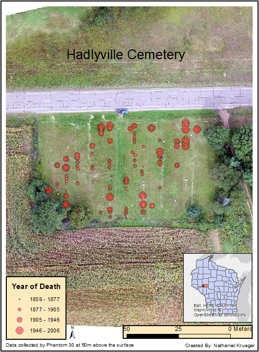
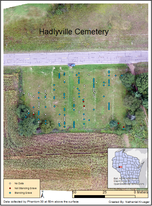
         Figure 8 below is a screenshot that shows where the survey locations were, meaning where the house or apartment was from. This can all be done from with the Survey 123 site. This can easily be turned into a map using illustrator or by importing it into ArcMap. Even the most inexperienced user could use this program by following the directions that were laid out in the tutorial.

Figure 8

        Figure 8 below is a heatmap of the survey locations. Due to the fact that the survey locations were so spread out there is really not a lot of significance displayed in figure 8. Though if there were more surveys done in different areas of the towns this illustration would be much more effective.

Figure 9

 Conclusion

          Survey 123 is a very effective way of creating a survey. It is extremely professional and it will definitely have many applications in the future. The surveys are easy to use and take, meaning that they do not take the survey taker long at all. From there the data is displayed by the program very nicely, it is easy to see the distributions of data and what they mean. This application has endless uses in the geography discipline. Surveyors could use it to ask if what they are doing is effective or what they could be doing differently.

Sources

https://learn.arcgis.com/en/projects/get-started-with-survey123/lessons/share-your-survey-data.htm

https://learn.arcgis.com/en/gallery/

https://learn.arcgis.com/en/projects/get-started-with-survey123/

Navigation Map

Introduction

    

          The main goal of this lab was to become familiar with navigation maps and how they are made, in an effort to be prepared for a upcoming exercise. In this lab a number of different coordinate systems and data projections were used, some show a drastic difference, while others are very similar. Some coordinate systems skew how the landscape actually is, this could lead to issues in a navigation map, so it is essential to make sure that a correct projection and coordinate system is used. 

           A projected coordinate system is defined on a two-dimensional surface and is based on a geographic coordinate system. This basically means that projected coordinate systems are best suited for navigational maps. In Map 1 below the coordinate system was WGS_1984_Web_Mercator_Auxillary_Sphere and in Map 2 the coordinate system used was NAD_1983_HARN_WISCRS_EauClaire_County_Meters. Map 2 was projected in "Lamber_Conformal_Conic" and Map 1 had the "Mercator_Auxillary_Sphere." Each coordinate system used did a good job of ensure data in integrity, meaning there was not much if any skewing in the data.

Methods

          Before the Navigation maps were created, the class took something called a pace count. The pace count used for this exercise was the number of paces it took to go 100 meters. This was done to the south of Philips hall on the sidewalk, starting near the southeast corner of the building and walking towards the southwest corner, and then back again to ensure that the numbers match up each time. This will come into play down the road because if someone wants to correctly use a navigation map, one must know how far they are walking and the scale of the map so they can tell if the desired destination is closer or further away from where they wanted to go. For each 100 meters walked, a pace count of 60 was recorded, meaning that every 60 steps, 100 meters is covered. 

Figure 1

       

   

           Next came the creation of the navigation maps using ArcMap. The first step was to add the navigation boundary, the Eau_Claire_West_SE and the 2ft contours from the Priory geodatabase which was copied over from the Share folder in the Q drive. Right away it is notable that the 2ft contours are not usable in this context, one would not be able to navigate because the contours take up too much of the image. Under the search menu, contours was searched and the results are displayed to the left. The spatial analyst tool was selected which is the second tool in the list. 

Figure 2

         

         

           To the right is the contour tool that was used, the input features was a feature class that was created inside of the geodatabase that was clipped for the specific area just outside of the navigation area. The output location was set to the geodatabase, this is an essential step, if the output location is wrong there may be no way to tell where the contour went after running the tool. The contour interval was set to 3 meters, more than four times larger than the initial contours that were offered for use. Changing the contours used opened the map up considerably for the viewer while still showing the increases in elevations that are associated with the UW-Eau Claire priory navigation area. From here the page view was changed to layout and also changed to 17 inches wide by 11 inches high, which is the correct size for printing of the maps. Then finally all of the cartographic fundamentals were accounted for including data sources, coordinate systems, and the projections. 

Results

Map 1

          Map 1 used the WGS_1984_Web_Mercator_Auxiliary_Sphere coordinate system and it displayed much in the same way as the coordinate system used in Map 2. The scale on Map 1 is slightly smaller than in Map 2, meaning that it is not zoomed in quite as far, though the grid is very detailed.

Map 2

          Map 2 used the coordinate system NAD_1983_HARN_WISCRS_EauClaire_County_Meters, this was a reletively easy choice becaue the navigation area lies within Eau Claire County. From here using a Lambert Conformal Conic map projection ensured that the map would have accurate direction and also that the features on the earth would not appear skewed or distorted. The grids on Map 2 are larger than in Map 1, they are spaced out at 50 meters. That being said, Map 1 would be a better option if the user had not previously been to this area.

          There are only a few slight differences between figure 1 and figure 2. The coordinate systems and projections are different along with the size and spacing of the grids. Additionally the orientation of the labels varies in each map. In Map 2 the labels are horizontal on the on the vertical axis and in Map 1 the labels are vertical on the vertical axis. Both labels remained horizontal on the on the horizontal axis.

           Both maps display the differences in elevation well. The east portion of the map clearly has the most drastic changes in elevation, while just to the east of that hill there is just a gradual slop. In the east half of the navigation area that is a steep incline, leading to the vegetation, where the elevation again evens out slightly. The northeast portion of the navigation area also shows large changes in elevation, though it is not as large as the elevation on the east edge, it is still a sizable hill.

          The structures in the photo are in the far east portion of the map, and slightly to the southwest of the center of the map. There is a road running north-south on the east portion of the map and it appears to be a county road. There is a highway with a clear median in the north portion of the map that runs northwest to southeast. The only large, continuous stand of forest lies in the eastern portion of the map and there is also a small pond just to the south of the highway in the upper portion of the map.

Conclusion

         This exercise was very beneficial in understanding how navigation maps are created. It should be noted that navigation maps are designed to do just that, help someone navigate. For this reason the maps should only contain what is necessary to navigate the area. This is why a locator map was left out, due to the fact that if someone is here navigating the area, they know where they are already. Navigation maps are useful for someone who may not have the money to spend several hundred or even thousands on a GPS. This is how things were done in the past and it is a skill that is necessary in this field.

Sources

http://resources.arcgis.com/en/help/

http://webhelp.esri.com/arcgisdesktop/9.3/index.cfmTopicName=Defining_a_shapefile%27s_coordinate_system     

Cartographic Fundamentals

Part 1: Map of my Terrain 


         Map making is an essential skill to have, knowing what needs to be included in a map and displaying data correctly and accurately is fundamental base in geography. Every map should include a north arrow, scale bar, locator map, a watermark and data sources. The data in figure 1 was collected near the beginning of the semester and it represents a homemade terrain model at a small scale. The model was made in a sandbox and the data was recorded and brought into Microsoft Excel and then ArcMap and finally ArcScene. Figures 2-5 were collected at the Hadlyville Cemetery using a DJI Phantom 30 at an altitude of 50 meters. Hadlyville cemetery is located in the southwest portion of Eau Claire county. The purpose of this lab is to be able to correctly make and display maps with data that was collected personally and then also with other data sets that were provided.

Figure 1

          Displayed above in Figure 1 is data that relates to the previous lab in which a elevation terrain model was constructed and a survey was completed. The map in the upper left hand corner was generated in ArcMap and it is a hillshade over laid with a spline of the sandbox data. In that illustration the elevation changes are noticeable, but not to the same extent as the other four illustrations below which came from ArcScene 3D. The four images in the bottom of figure one show how the sandbox looked from each angle all the way around. Each angel does its part in giving the viewer a more realistic idea of what the real sandbox had looked like. In each angle the origin or (0,0) changed and the the orientation of the north arrow was shifted to ensure data integrity. The high elevation values are depicted by red and the low elevation values are a green/ blue. The largest mountain/ hill in the elevation model is in the northeast portion of the sand box and it is clearly shown in all five of the maps. The crater in the northwest portion of the sandbox showed up nicely, especially in the 3D ArcScenes. The goal was to model the indentation after a erupted volcano and it showed up clearly. On the southern area of the maps there is a valley that spans most of the sandbox and just to the south of that there is a small rise in elevation that goes to the extent of the survey area.

Part 2: Maps using data with Attributes, Hadlyville Cemetery

Figure 2

          Figure 2 above illustrates the year of death of each person by grave. There is a somewhat even distribution of the year of death. Though the 1946-2006 tend to catch the viewers eye because they have the largest proportional symbol. The rows in the cemetery are pretty apparent here, though the graves are not even spaced. Year of death is an important variable to look at here because there may be links between age of the grave and if the stone is still standing, also the family location, and the specific year of death. There is no true spatial pattern of the year of death in the cemetery as a whole. To clarify there are years of death from 1946-2006 in every corner of the cemetery, similarly there are also years of deaths from 1859-1877 fairly evenly distributed throughout the cemetery.

Figure 3

           Figure 3 shows whether or not there was a grave stone at the grave sight or not. The first issue to be discussed here is why some come back as no data. To be honest, there is no explanation for why there is no data, either the headstone was standing or it was not. This would be a good question to ask whoever completed the data collections. This is only brought up because there is a significant portion of the cemetery that has no data. For the most part, the majority of graves are standing, there is only five graves that were marked as not standing graves. There are two in the east portion of the map, two in the center and one in the west side of the cemetery. Now referring back to figure 1, it was important to check if the graves that were not standing were older graves because that could account for them not being there. The headstones have went through over 100 years of Wisconsin Climate and this most likely accounts for the reason they are not there, also it could have been that in that time head stones were not as popular due to financial strain.

Figure 4

          Figure 4 is a map that shows the last name of each person buried at that grave. This is something that is very interesting when looking at cemetery's because family members are often buried together. In the northeast portion of the map there are five Mcdonalds, in the further northeast section there are three Sessions. After further examination it is clear to see that there are many other names that have multiple graves in the cemetery. This is because families often buy multiple grave sites so they can be buried near loved ones. One interesting thing to note is that in the southwest corner of the cemetery there are several Hadley's, the significance is that this could have been the founder of the cemetery or possibly even Hadleyville. Referring back to figure 2, the graves do match up as being from 1859-1877 which is the oldest data that is recorded.

Figure 5

           Figure 5 shows the specific year of death for each grave that the data was available. This is significant because it can give a better idea of the links between group family burials, grave stone condition and other information than just the proportion symbols map that is shown in figure 1. In the northeast corner of the cemetery there are four Sessions buried, the reason attention is being brought to this is to note that the burial lots were most likely purchased at the same time. The top Sessions was buried in 1904, then the most recent is 2006. Over 100 years apart and that family is still getting buried near other family members. Another pattern that should be noted is that in the western third of the cemetery the majority of the years of death are from pre 1900. As stated when discussing figure 2 there is not a clear spatial representation of this, but that is because the proportional symbols for years of death post 1900 are significantly bigger and therefore it is easy to assume they carry more weight, though they do not. 

Sandbox Survey Part II: Visualizing and Refining the Terrain Survey

Introduction 

          In last weeks lab, a one meter by one meter sand box was surveyed in small teams and 400 data points were collected after creating a unique elevation model. The top of the wood on the sandbox was considered sea level and received values of 0. The sand box was fitted with a x, y grid to ensure correct, accurate data collection. Picture 1 below shows the method of data collection and also shows the hill in the bottom left corner that is displayed in the interpolations. To follow up on last week's lab, our x, y, z data that was collected on paper was brought into Microsoft excel and normalized in a way that in was compatible with ArcMap. Normalizing data involves  organizing the data into rows and columns in a manner that is uniform regarding positive and negative values and helps to improve the accuracy and reliability of the data. Data normalization is the first essential step in correctly getting the data into ArcMap. If the data is not correctly normalized it will not be able to be opened in ArcMap.

Picture 1

          The goal of this lab is to bring life to the data in the form of maps constructed on ArcMap and Arc Scene. The data interpolation done in lab was done to fill in values that were not collected. This is a way to get a map of a survey area without collecting data at a level that would not be achievable. The 400 points collected in the elevation model sandbox were displayed in various 2D and 3D models using different methods of interpolation techniques. Interpolation helps to create a continuous data surface, rather than just the points that were collected. In this lab five different methods were used to display the data, Inverse Distance Weighted (IDW), Kriging, Natural Neighbor, Triangular Irregular Networks (TIN), and Spline.

Methods

          The lab began with creation of a folder in the Q drive and a geodatabase inside of that to ensure a safe spot to save the data that also had adequate storage space. From here the x,y ,z data that was collected and entered into ArcMap was imported into the Geodatabase. As stated earlier the data was normalized with the correct decimal places and values. Next, the data was brought into ArcMap by adding the "X,Y," data under the file tab. After the data was displayed in ArcMap as points, the steps for interpolation were able to be completed.

          IDW manipulates a raster surface using inverse distance weighted in order to fill in the data between the points collected from the survey. This is done by the average being collected around the outside of a cell in order to determine the value of each point. This method of interpolation does not make defined valleys and peaks due to the fact that there is an average taken to calculate the unknown data values. This method is affected by how close a point is to the center of the cell that is being interpolated, meaning that the closer a point is to the center the greater the affect it will have in the process of averaging out the data. IDW best serves a purpose that is a larger scale rather than the small scale application of this lab. 

          Kriging interpolation is a technique that uses the Z-values patterns to calculate the missing values and to create a continuous surface. Kriging uses a interpolation method that relies on spatial corrections such as distance to explain differences in elevation. This method of interpolation is best suited for areas with drastic elevation changes because the rigidness of the model will be less noticeable in that setting.

         The Natural Neighbor interpolation model involves applying all perimeter values to create the value near there. This model is somewhat similar to other methods and provides a relatively smooth surface. Though it should be noted that if there are more than 15 million data points another technique should be used.

          The Spline interpolation technique uses an algorithm in order to cut down on rough elevation differences. It is visibly the smoothest when discussing the differences in elevation throughout the model. By using a mathematical algorithm to calculate the missing data values, there is a smooth surface created because missing data values are filled in as if there was uniform contours between the data points collected. In contrast to the kriging method, spline uses the max and min values in order to create a continuous and fluid display.

          Finally a TIN interpolation is used to create digital elevation surface model by connecting data points triangularly. While this method appears to be very rough and not smooth, it is very accurate in displaying elevation data. This model is effective on a small scale when there is not a lot of data values.

         After the completion of each technique in ArcMap the data was then brought into ArcScene. This is where the data was created into a 3D image. This is essential in surveying because it is an effective way to convey data to a third party because the changes in elevation can be clearly noted.

Results/ Discussion

          Displayed below are five figures which display the data that was collected in the sandbox, each displays a different interpolation method. Each method has its differences, some are slight while others are more drastic. As discussed in the methods section above, each technique is designed for a specific use. Many of the methods below could have been more accurate had more data points been collected and it would be interesting to see how these models would change as more data points were added and taken away. Each of the five figures below are formatted in the same way, meaning the the 0,0 are the same in each display. Also the Arc Map illustration are on top and the later completed Arc Scene interpolations are on the bottom.

        

Figure 1

TIN as pictured above by figure 1 does a nice job of showing the features, especially when in a 3D setting. In the bottom image, in the lower right hand corner the slight hump is clearly apparent, while it was considerably less notable in the IDW pictured in figure 3. TIN works by making triangles between the data points, this accounts for the jaggedness of the image, but this is also the reason the features are easy to see. This would be a good route to choose to just show the changes in elevation and then followed up with a more real world, smooth interpolation such as Spline.

Figure 2

Spline interpolation relies on the data points in a similar manner to natural neighbor which is discussed below. A mathematical equation is used to calculate the missing values. While spline may add an almost too defined point to some of the areas, this is the technique that was most like what was created in the sandbox. This could be different for other groups, due to the fact that the spline tool attempts to limit the amount of severe curves.

Figure 3

Due to what was discussed in the methods section, the IDW is not the correct interpolation technique to use in this setting. This method leaves a rather jagged appearance. For example the ridge in the bottom of figure 3 appears to have multiple peaks, rather than one peak as it was designed before the survey.

Figure 4

Natural neighbors is an okay method of portraying this data set, though the area between the data points collected were just smoothed out, therefore losing some of there characteristics. There is not a real defined valley as it was designed, hence why this is not the number one choice of interpolation used in this exercise.

Figure 5

Kriging uses a very advanced mathematical equation in order to calculate the missing values between data points. This is not a bad method for this survey, and this technique of interpolation is one that has many real world applications due to the sophisticated equation used to calculate the values.

Conclusion

          Having data displayed in a visual manner is essential in understanding what is being portrayed. Using these models rather than discussing a table makes it much more interactive and beneficial for the people viewing.  Fortunately for the group the data collected was very good the first time so no additional data manipulation was necessary. Looking back the data could have been more drastic in the aspect of elevation changes.  This sand box activity helped to display a x, y, z table in both 2D and 3D models, a skill that is essential in moving forward in this field. Interpolating data is a way to basically fill in the blanks between data in a continuous manner. After completion of this exercise, the spline method of interpolation is the most accurate at this scale and with this amount of data points. This is a useful skill to have because it showed how to easily collect and display data on a real world small scale. Granted in a real world setting data will not always be collected in this detailed of a manner, but rest assured even with a less detailed survey interpolation can be effective. Interpolation is something that is used in so many different applications. Often in the real world companies do not have time to survey every single person, or to collect data that is accurate down to the centimeter and that is where interpolation helps to fill in the gaps.














Sources

http://resources.arcgis.com/en/help/

Creating a Digital Elevation Surface Model

Introduction

           Sampling is a technique that is used to get a general idea of something by only taking data from certain areas rather than the whole. There are three main ways to sample an area, random, systematic and stratified. Random sampling is just as it sounds, each data value has a equal chance of being selected, a efficient way to do this is with a number generator. Systematic sampling is done by taking a sample at a set interval, for example every two inches, or maybe every 5th house. The third and final sampling method to be discussed is stratified. There is both systematic and random stratified sampling, and each has there own applications. The goal of the week one activity was to encourage students to work together in order to grid out and survey a student created terrain. From here, the data was collected first on paper and later entered into Microsoft Excel. The size of the sand box was approximately one square meter, each group was tasked with creating a unique digital elevation surface. In the beginning of the lab there were no official guidelines on how to begin, the sandbox was shown to the class and the tools were laid out.  The ultimate objective of this lab is to collect sample data, enter it in to Excel and in later weeks the data will be analyzed in ArcMap.

Methods

         Our study was completed on Monday, January 30th from 3:00 pm until 4:30 pm. The square meter sand boxes were located south of the steam near the garden and across the road to the east from the Philips garage. The sampling technique that my group decided would be the most accurate was the systematic method. Due to the fact we had a nearly perfect square meter to work with, the systematic method of sampling works really nicely because there is no discrepancies when measuring the grid on the box. To assist in data collection and documentation a variety of tools were used including tape, string, thumb tacks, notebooks, meter sticks and a cell phone. The group decided that zero elevation, which is sea level was going to be flush with the top of the wood on the sandbox which is where the string was attached. Negative values were referred to as below sea level and positive values accounted for above sea level. The sandbox had a grid that was 20 x 20, this equates to 400 data points collected. The data was collected from left to right, starting at the bottom left of the sandbox which was coordinate 0,0. Using a coordinate system helped to keep the data organized.

Results/ Discussion

          As stated above, the sandbox had a grid that was 20 x 20 and there were 400 data points collected from the sandbox in order to ensure enough data points that the changes in elevation would be noticeable on the map, but not so many points that this exercise became overwhelming. The data points collected were approximately 5 cm or 1.96 inches apart. The terrain elevation data that was collected was done in centimeters, the max value above 0, or sea level was 4 an the minimum value, or below sea level was -8.

          There were a few issues that did occur during the lab. For starters some of the sand was frozen solid which dictated partially where our changes in elevation had to be placed due to the fact that we did not have a shovel. Next as data collection was in full swing, the sting used to grid out the sandbox would sometimes loosen up. A better way to do this would have been with three inch nails that would not pull out rather than flimsy thumb tacks, and another improvement would have been to use string that does not have any pliability, that way as the surveyor there is no concern that the string will stretch and become slack. Also looking back, additional sand would have helped to make the exercise run smoothly. The frozen ground, coupled with a half full sand box accounted for much of our values being below 0.

Conclusion

Sampling is effective in a spatial setting because with enough sample points an accurate map of elevation can be created. In a way the method used to grid out this sandbox is similar to how the Public Land Survey System (PLSS) maps out land into 40 acre squares, it is time efficient and accurate. When looking at the numbers that were gathered throughout this exercise, it certainly would not have been a bad idea to add a little more data to our sampling. What that means is making the grid 25 x 25, which would be 625 data points. The smaller distances between each elevation taken would allow for better visualization of the changes in elevation. That being said, the data collected was certainly adequate, as it did show the changes in elevation, it just could have been more detailed had the smaller grid been implemented.

Sources

• http://www.rgs.org/OurWork/Schools/Fieldwork+and+local+learning/Fieldwork+techniques/Sampling+techniques.htm